
Building a Real-Time Satellite Tracking Pipeline with Spark Structured Streaming
Leverage the latest features of Apache Spark 4 to stream, process, and visualize satellite orbit telemetry using public TLE data and real-time processing techniques.


✨ Introduction
If you’re into space, objects in orbit, and data… I have a treat for you today! I have really enjoyed getting more familiar with Pyspark 4’s Custom Data Sources, and recently wanted to explore more datasets for real-time streaming use cases.
One day, I stumbled across this TLE API, a public API providing data from CelesTrak, a non-profit that hosts data for the space community.
Satellite data is super compelling for real-time use cases and they’re constantly moving. Tens of thousands of these objects (over 63k known to the public in fact) are in orbit for a variety of purposes: communication satellites like Starlink, weather satellites, navigation/GPS satellites, reconnaissance satellites, and even natural satellites like asteroids or the moon.
In this post, we’ll build a real-time streaming pipeline using Apache Spark to track satellites using Two-Line Element (TLE) data, predict their near-future positions, and visualize their motion in 3D.
🔌 Data Sources
First, we need to identify our data sources. How does one get this data, much less determine a satellite's position or velocity? If you work in space telemetry or are already a hobbyist, you probably already know the answer; for the rest of us, let’s take a moment to understand a piece of data known as TLE (Two-Line Element).
🏛️ A Brief History of TLE
TLEs (Two-Line Element Sets): The standard format for describing satellite orbits.
It’s called “two-line” because it literally consists of two lines of 69-character data that encode orbital elements necessary to calculate a satellite’s position and velocity at a given time.
Format example:
ISS (ZARYA)
1 25544U 98067A   24101.21315433  .00002243  00000+0  48609-4 0  9991
2 25544  51.6392  59.7121 0003000  73.4153 286.7121 15.50011348397460
The US Air Force developed this format, and it was adopted by NORAD (North American Aerospace Defense Command) during the Cold War to track objects in space. It was designed to be machine-readable, which at the time meant early mainframe systems and punch cards!
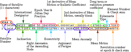
For details on each field encoded into this format, check out the Wikipedia for TLE.
Public Sources
TLE is publicly available from sources like:
TLEs are updated frequently and can be streamed periodically.
Simplified Perturbations Models (SGP/SDP)
Unfortunately, TLE cannot tell us a satellite's position or velocity by itself. For this, we need to use an established mathematical algorithm like SGP4 or SDP4, which are known as Simplified Perturbations Models.
Don’t worry—we don’t have to be a rocket scientist to understand this. Think of it as a function of two inputs—the TLE and a timestamp. In other words, we can say, “Based on the TLE, where will this object be at this point in time?”
🏗️ Architecture Overview
Ingestion: TLE data is streamed in with a custom spark source we build that calls the HTTP TLE API, ingesting TLE for one or more satellites.
Processing: Transform the satellites’ state into a usable format (coordinates we can plot relative to Earth).
Prediction: Use SGP/SDP models combined with TLE to predict the satellites' position and velocity at various points in time.
Visualization: 3D plots in matplotlib.
📡 Ingesting Satellite Data
We’ll cover a lot of code here, but I’ll break it down step by step. As a prerequisite, know that this will require Pyspark 4 (I used pyspark==4.0.0.dev1 at the time of this writing).
Project Setup
First, we will bootstrap the project with some dependencies. I am using uv to manage the Python project.
uv init --python python3.11 spark-ingest-tle
cd spark-ingest-tle
uv add \
  grpcio \
  grpcio-status \
  pyspark==4.0.0.dev1 \
  astropy \
  sgp4 \
  matplotlib \
  pandas
Now for the main code, let’s take care of our imports and setting up the Spark Session:
import pandas as pd
import matplotlib.pyplot as plt
import numpy as np
from pyspark.sql.datasource import DataSource, DataSourceStreamReader, DataSourceReader, InputPartition
from pyspark.sql.types import StructType
from pyspark.sql import SparkSession, functions as F

import requests
from datetime import datetime, timedelta

spark = SparkSession.builder.appName("SatelliteStream").getOrCreate()
Implementing Streaming Reader
To support streaming with our custom source, we must implement the DataSourceStreamReader from PySpark. This provides the interface we must use to implement how partitions are generated, how data is read, and how offsets/checkpoints are defined.
def fetch_tle_data(norad_id: str, api_key: str) -> dict:
    headers = {"Accept": "*/*", "User-Agent": "curl"}
    url = f"https://tle.ivanstanojevic.me/api/tle/{norad_id}"
    response = requests.get(url, headers=headers, params={"api_key": api_key})
    response.raise_for_status()
    return response.json()

class SatellitePartition(InputPartition):
    def __init__(self, norad_id: str, name: str,tle_line1: str, tle_line2: str, tle_timestamp: datetime, size: int):
        self.norad_id = norad_id
        self.name = name
        self.tle_line1 = tle_line1
        self.tle_line2 = tle_line2
        self.tle_timestamp = tle_timestamp
        self.size = size

class SatelliteStreamReader(DataSourceStreamReader):
    def __init__(self, schema: StructType, options: dict):
        self.norad_id = options.get("norad_id").split(",")
        self.size = int(options.get("size", 5))
        self.timedelta = options.get("timedelta", "seconds=1").split("=")
        self.timedelta = {self.timedelta[0]: int(self.timedelta[1])}
        self.api_key = options.get("api_key", "DEMO_KEY")

    def initialOffset(self):
        """
        Return the initial offset of the streaming data source.
        A new streaming query starts reading data from the initial offset.
        If Spark is restarting an existing query, it will restart from the check-pointed offset
        rather than the initial one.

        Returns
        -------
        dict
            A dict or recursive dict whose key and value are primitive types, which includes
            Integer, String and Boolean.
        """
        return {}

    def latestOffset(self) -> dict:
        """
        Returns the most recent offset available.

        Returns
        -------
        dict
            A dict or recursive dict whose key and value are primitive types, which includes
            Integer, String and Boolean.
        """
        # Fetch the TLE data for each of the given satellites
        offsets = {}
        for norad_id in self.norad_id:
            tle = fetch_tle_data(norad_id, self.api_key)
            tle_line1 = tle["line1"]
            tle_line2 = tle["line2"]
            name = tle["name"]
            tle_timestamp = tle["date"]
            offsets[norad_id] = {"name": name, "tle_line1": tle_line1, "tle_line2": tle_line2, "tle_timestamp": tle_timestamp}
        return offsets

    def partitions(self, start: dict, end: dict):
        partitions = []
        for id, val in end.items():
            if id not in start:
                partitions.append(SatellitePartition(id, val["name"], val["tle_line1"], val["tle_line2"], val["tle_timestamp"], self.size))
            else:
                if start[id]["tle_line1"] != val["tle_line1"] or start[id]["tle_line2"] != val["tle_line2"] or start[id]["tle_timestamp"] != val["tle_timestamp"]:
                    partitions.append(SatellitePartition(id, val["name"], val["tle_line1"], val["tle_line2"], val["tle_timestamp"], self.size))
        return partitions

    def read(self, partition: SatellitePartition):
        from datetime import datetime, timedelta
        from sgp4.api import Satrec, jday, SGP4_ERRORS

        satellite = Satrec.twoline2rv(
            partition.tle_line1,
            partition.tle_line2
        )

        for i in range(partition.size):
            ts = datetime.now() + (timedelta(**self.timedelta) * i)
            jd, fr = jday(
                ts.year,
                ts.month,
                ts.day,
                ts.hour,
                ts.minute,
                ts.second,
            )

            e, r, v = satellite.sgp4(jd, fr)
            if e != 0:
                e = SGP4_ERRORS.get(e, 'Unknown error')
            r = {"x": r[0], "y": r[1], "z": r[2]}
            v = {"x": v[0], "y": v[1], "z": v[2]}
            yield (
                ts,
                r,
                v,
                e,
                partition.norad_id,
                partition.name,
                datetime.strptime(partition.tle_timestamp, "%Y-%m-%dT%H:%M:%S%z"),
                partition.tle_line1,
                partition.tle_line2,
                jd,
                fr
            )
Let’s break it down.
It starts with the constructor __init__ which is where we’ll grab any custom options we’d like to define.
    def __init__(self, schema: StructType, options: dict):
        self.norad_id = options.get("norad_id").split(",")
        self.size = int(options.get("size", 5))
        self.timedelta = options.get("timedelta", "seconds=1").split("=")
        self.timedelta = {self.timedelta[0]: int(self.timedelta[1])}
        self.api_key = options.get("api_key", "DEMO_KEY")
These are the options we can pass in like so: spark.readStream.option(“norad_id”, “33499”)…
Disregard the schema argument here for now. We won’t be using this since our data source will have a fixed schema based on the TLE API.
initialOffset and latestOffset
Offsets are how Spark Structured Streaming keeps track of which data has already been processed in a stream. Think of it like a bookmark, or a cursor, in database terms.
When developing your own custom pyspark source, you get to define what these offsets look like. How you choose to model this will heavily depend on the system(s) that your source is consuming; in a durable stream like Kafka or Kinesis, this would involve storing attributes like the sequenceNumber and shardId. In our case, the TLE API doesn’t offer a way to retrieve previous data, so we just won’t worry about replayability; however, the API does return a date field, and we can check if the date, or the contents of line1 or line2, have changed since the last time we fetched the TLE.
Our Offset Data Model
Since I want to compare these values each time I poll the API, I’ll store these things in my offsets. Therefore, the offsets will look like this:
{
  satellite_id: {
    "name": name,
    "tle_line1": tle_line1,
    "tle_line2": tle_line2,
    "tle_timestamp": tle_timestamp
  },
  ...
}
Using the satellite ID (NORAD ID) as a key allows us to track multiple satellites in the same stream, which will be useful and more scalable later on.
Initial Offset
Our class’s initialOffset function will initialize the offset data for new streams. Once a stream is started and successfully processed, the offsets will be written to Spark checkpoints and no longer use the initialOffset function. In our case, we haven't fetched the TLE data yet, so we’ll initialize the offset to an empty dict.
Latest Offset
    def latestOffset(self) -> dict:
        # Fetch the TLE data for each of the given satellites
        offsets = {}
        for norad_id in self.norad_id:
            tle = fetch_tle_data(norad_id, self.api_key)
            tle_line1 = tle["line1"]
            tle_line2 = tle["line2"]
            name = tle["name"]
            tle_timestamp = tle["date"]
            offsets[norad_id] = {"name": name, "tle_line1": tle_line1, "tle_line2": tle_line2, "tle_timestamp": tle_timestamp}
        return offsets
The latest offset should return the most recent offset available for our source. This is where we will actually make the HTTP request to fetch TLE data for each of the satellites being tracked.
As you recall from the class constructor, we allow the user to pass in multiple satellite IDs separated by commas.
Partitions
If offsets act like pointers for the source, then the class's partitions method involves taking Point A and Point B (start/end) and dividing them into one or more logical partitions.
The read() method will be invoked for each partition we return by our source.
In my case, I’d like to only emit new data when there is new/updated TLE information for the satellite, and I’d like to generate a partition for each satellite. Thus, I’ll model my partition like so:
class SatellitePartition(InputPartition):
    def __init__(self, norad_id: str, name: str,tle_line1: str, tle_line2: str, tle_timestamp: datetime, size: int):
        self.norad_id = norad_id
        self.name = name
        self.tle_line1 = tle_line1
        self.tle_line2 = tle_line2
        self.tle_timestamp = tle_timestamp
        self.size = size
Then, the partitions are generated by looping over the end offset (latest offset) and comparing it to the start offset (last offset that we processed). If there is new data, we’ll generate a partition.
    def partitions(self, start: dict, end: dict):
        partitions = []
        for id, val in end.items():
            if id not in start:
                partitions.append(SatellitePartition(id, val["name"], val["tle_line1"], val["tle_line2"], val["tle_timestamp"], self.size))
            else:
                if start[id]["tle_line1"] != val["tle_line1"] or start[id]["tle_line2"] != val["tle_line2"] or start[id]["tle_timestamp"] != val["tle_timestamp"]:
                    partitions.append(SatellitePartition(id, val["name"], val["tle_line1"], val["tle_line2"], val["tle_timestamp"], self.size))
        return partitions
Read and Predict
Next, we’d like to predict the position and velocity of the satellite using math. We’ll encapsulate the gory details in our custom source so users don’t have to look like this Charlie Day meme:
One of the most important notes about the read() method is that it should be stateless. You should not access class member variables or try to change the class’s state from within this function. This also means that any modules that need to be imported should be imported from within this function.
Our read function will take the TLE data and calculate the object's position (r) and velocity (v). To make things more interesting, we will calculate not only for the current time but also for N future intervals, therefore predicting where the satellite will be in the near future.
    def read(self, partition: SatellitePartition):
        from datetime import datetime, timedelta
        from sgp4.api import Satrec, jday, SGP4_ERRORS

        satellite = Satrec.twoline2rv(
            partition.tle_line1,
            partition.tle_line2
        )

        for i in range(partition.size):
            # SGP requires the timestamp to be in Julian date format
            ts = datetime.now() + (timedelta(**self.timedelta) * i)
            jd, fr = jday(
                ts.year,
                ts.month,
                ts.day,
                ts.hour,
                ts.minute,
                ts.second,
            )

            e, r, v = satellite.sgp4(jd, fr)
            if e != 0:
                e = SGP4_ERRORS.get(e, 'Unknown error')
            r = {"x": r[0], "y": r[1], "z": r[2]}
            v = {"x": v[0], "y": v[1], "z": v[2]}
            yield (
                ts,
                r,
                v,
                e,
                partition.norad_id,
                partition.name,
                datetime.strptime(partition.tle_timestamp, "%Y-%m-%dT%H:%M:%S%z"),
                partition.tle_line1,
                partition.tle_line2,
                jd,
                fr
            )
Finishing the Custom Data Source
To put it all together for our custom data source, we now need to implement the DataSource class, which is the top-level wrapper.
class SatelliteDataSource(DataSource):
    """
    A data source for satellite data.
    """

    @classmethod
    def name(cls):
        return "satellite"

    def schema(self):
        return """
            ts TIMESTAMP,
            pos STRUCT<
                x:DOUBLE,
                y:DOUBLE,
                z:DOUBLE
            >,
            velocity STRUCT<
                x:DOUBLE,
                y:DOUBLE,
                z:DOUBLE
            >,
            e STRING,
            norad_id STRING,
            name STRING,
            tle_timestamp TIMESTAMP,
            tle_line1 STRING,
            tle_line2 STRING,
            jd DOUBLE,
            fr DOUBLE
        """

    def streamReader(self, schema: StructType):
        return SatelliteStreamReader(schema, self.options)
Finally, we can register the source so Spark knows about it.
spark.dataSource.register(SatelliteDataSource)🤩 Using the Custom Source
To use the source, we write some familiar, idiomatic, Pyspark code:
df = (
    spark
        .readStream
        .format("satellite")
        .option("norad_id", "25544,33499")
        .option("size", "5")
        .option("timedelta", "minutes=1")
        .option("api_key", "DEMO_KEY")
        .load()
)

# Processing the stream
q = (
    df
        .writeStream
        .format("console")
        .outputMode("append")
        .trigger(once=True)
        .start()
        .awaitTermination()
)
Processing
Now that we have a streaming source that can read TLE data for multiple satellites, we can build processing use cases around this.
There’s all sorts of processing we could do against this TLE data: anomaly/drift detection, collision prediction, data visualization, etc.
Let’s examine a simple processing use case of transforming the data into Earth-centered, Earth-fixed (ECEF) coordinates and then visualizing the data in a 3D plot.
Convert TEME to ECEF Coordinates
The raw position coordinates we have for now are in the True Equator, Mean Equinox (TEME) coordinate system. We need to convert these into ECEF coordinates to plot them in relation to the Earth.
This is a classic use case for data transformations. Let’s write a helper function, which we can later use as a User-Defined Function (UDF).
from astropy.time import Time
from astropy.coordinates import TEME, ITRS
from astropy import units

# Convert TEME to ECEF
def teme_to_ecef(rx, ry, rz, jd, fr):
    teme_position = TEME(
        rx * units.km,
        ry * units.km,
        rz * units.km,
        obstime=Time(jd + fr, format="jd")
    )
    ecef_position = teme_position.transform_to(ITRS(obstime=teme_position.obstime))
    return ecef_position.x.value, ecef_position.y.value, ecef_position.z.value
Data Visualization
Static visualization can be done with matplotlib. We will use a 3D scatter plot to represent satellite positions and a wireframe sphere to represent the Earth.
Let’s put this in a helper function to be reused:
from pyspark.sql import DataFrame
import matplotlib.cm as cm

def visualize(df: DataFrame):
    pDF = df.toPandas()
    pDF["color_id"] = pd.factorize(pDF["norad_id"])[0]

    # Generate a color map for unique norad_ids
    unique_ids = pDF["norad_id"].unique()
    id_to_color = {
        norad_id: cm.viridis(i / len(unique_ids))
        for i, norad_id in enumerate(unique_ids)
    }

    # Convert TEME to ECEF
    pDF["x_ecef"], pDF["y_ecef"], pDF["z_ecef"] = zip(*pDF.apply(lambda row: teme_to_ecef(
        row["pos"]["x"], row["pos"]["y"], row["pos"]["z"], row["jd"], row["fr"]
    ), axis=1))

    # Plotting
    fig = plt.figure()
    ax = fig.add_subplot(111, projection='3d')
    ax.set_xlim([-7000, 7000])
    ax.set_ylim([-7000, 7000])
    ax.set_zlim([-7000, 7000])
    ax.set_xlabel('X (km)')
    ax.set_ylabel('Y (km)')
    ax.set_zlabel('Z (km)')

    # Plot the Earth
    u, v = np.mgrid[0:2*np.pi:100j, 0:np.pi:50j]
    x = 6371 * np.cos(u) * np.sin(v)
    y = 6371 * np.sin(u) * np.sin(v)
    z = 6371 * np.cos(v)
    ax.plot_wireframe(x, y, z, color='blue', alpha=0.1)

    # Plot the satellites with different colors for each one
    for norad_id, g in pDF.groupby('norad_id'):
        ax.scatter(
            g["x_ecef"],
            g["y_ecef"],
            g["z_ecef"],
            color=id_to_color[norad_id],
            s=10,
            label=f"Satellite {norad_id}"
        )

    ax.legend()
    plt.show()
🚀 Putting It All Together
This is where we put it all together! We’ll read-stream TLE data for three satellites simultaneously, compute their position and velocity, predict where they will be at each minute over the next 4 hours, convert those positions to an ECEF coordinate system, and finally plot these predictions on a 3D visualization.
df = (
    spark
        .readStream
        .format("satellite")
        .option("norad_id", "25544,33499,46362")
        .option("size", "240") # 240 predictions
        .option("timedelta", "minutes=1") # 1-minute predictions. 240 x 1 minute = 240 minutes = 4 hours
        .option("api_key", "DEMO_KEY")
        .load()
)

# Processing the stream
q = (
    df
        .writeStream
        .outputMode("append")
        .trigger(once=True)
        .foreachBatch(lambda df, batch_id: visualize(df))
        .start()
        .awaitTermination()
)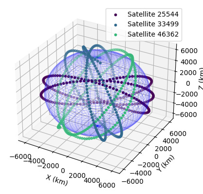
Result and Final Thoughts
Wow. Obviously, I am not the best at matplotlib, and this data visualization does leave some to be desired; however, it’s amazing how simple and idiomatic it is to build.
⚠️ Cautionary Comments
Although it’s quite easy to build your own custom sources now with Spark 4 and newer Databricks Runtimes. I would caution you to think very carefully about the following implementation choices:
What to use for offsets
Offsets are a critical piece of spark streaming. If your upstream source has any knobs or attributes that make it durable or replayable, you should definitely consider leveraging these in your source.
How partitions are created
The number of partitions your source generates from the partitions() method will directly impact the amount of parallel processing that Spark can do with its executors. Avoid having too few partitions if your dataset is very large, and avoid over-partitioning, which can lead to a Large Number of Small Files Problem.
NOTE: alternatively, if you don’t need partitioning, you can implement the SimpleDataSourceStreamReader instead of DataSourceStreamReader.
Avoid accessing state or mutating class members from the read() method. As a general rule of thumb, I try to avoid using the self keyword in this method.
Source Code
All of the source code is available on GitHub. I have also implemented support for batch reading on this source code, so take a look if you are interested in more than just streaming.